Simulated Annealing and Drawing Connections
Act I - The Challenge⌗
One day, out of the blue, our Algorithms 2 lecturer set us a problem and challenged us to devise an algorithm. The problem, available here, is as follows:
Given a set of $N$ items and a set of $M$ similarity scores between some pairs of items, devise an ordering of the set of items such that items that are more similar are placed closer together in the ordering.
To quantify this, the score of an ordering is defined as: $$\text{score}=100\times\frac{x-m}{-m} \quad\text{where}\quad x = \frac{1}{M N}\sum_{\text{pairs }(u,v)} \bigl|z_u-z_v\bigr|\log(1-s_{u v})$$ $$\text{and the constant} \quad m = \frac{1}{3M}\sum_{\text{pairs }(u,v)} \log(1-s_{u v}),$$ where $z_x$ is the index of item $x$ in the ordering and $s_{uv}$ is the similarity score between $u$ and $v$.
Your task is to find an ordering $z$ that maximises this score.
Our submissions had to be in Python. Our lecturer, being a Data Science Enjoyer, also allowed us to use numpy and pandas.
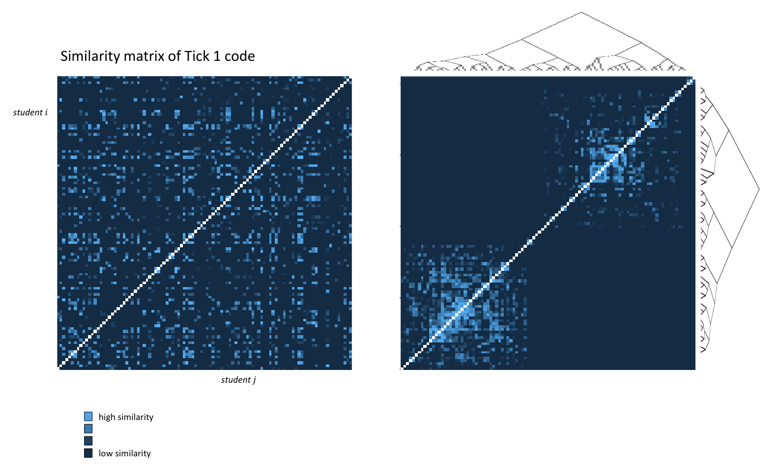
Our lecturer then showed us an approximate solution using Kruskal’s algorithm (for those who are interested, the algorithm builds and traverses a “Kruskal reconstruction tree”) and presented us with some pretty epic diagrams:

The Epic Diagrams(tm) presented during a lecture
So yeah, our goal is to get the light spots to be as “clustered” together as possible.
After looking at the problem for a bit, I began to wonder how well simulated annealing would perform.
Act II - The Algorithm⌗
But wait, what is simulated annealing?⌗
The Wikipedia page can explain it better than I do, but if I were to give a quick summary, it’s like a hill-climbing algorithm but modified to be more fuzzy so that you get a better solution in the long run.
The general idea is this:
- At the start, explore a bunch of different solutions across the solution space
- Go down one of the solution spaces that seem to be promising
- As you explore more and more solutions, start to pick off the obviously bad choices
- Towards the end, just try and optimise your current solution as much as possible
The reason this is called “simulated annealing” is that this algorithm lends many similarities to metal cooling in real life. In fact, some of the terminology we use is also borrowed from physics.
Energy⌗
How bad a solution is, is called its energy. As such, we want our solution to be in a low-energy state in the end.
We explore our solution space by randomly modifying the solution such that the energy is only affected by a slight amount. In our example, we can swap two random elements in our ordering, which produces a solution that is different, but not by much.
Temperature⌗
We also have another variable, called the temperature. The temperature represents how willing we are to risk keeping a modification that leaves the solution in a higher energy state. A high temperature means that we don’t care, whereas a low temperature means that we are unlikely to make this trade-off.
In the algorithm, the temperature starts off very high and gradually decreases over time following some function (that you can tweak) until it reaches zero.
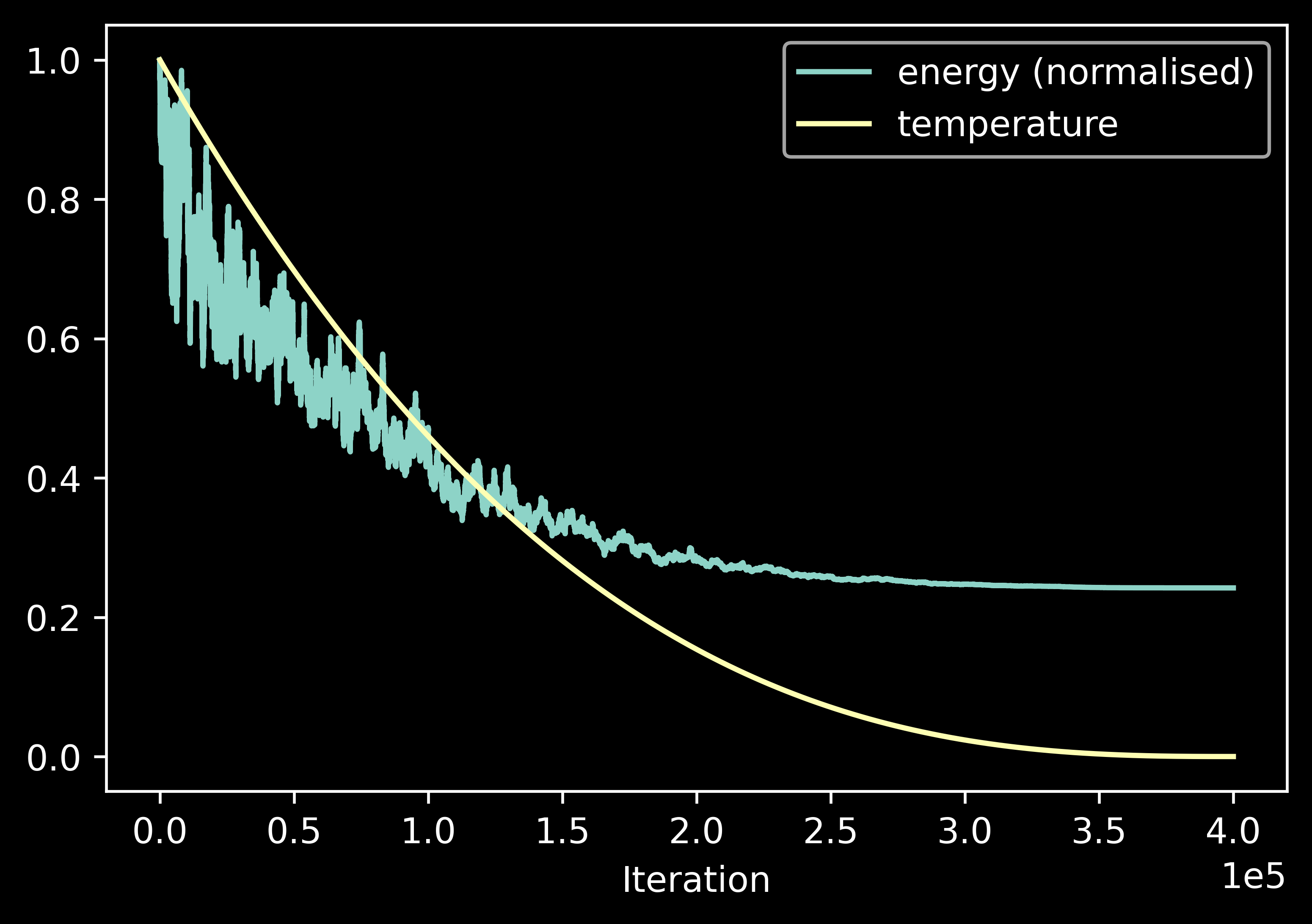
Here is a visual representation of how the energy and temperature change over time:

Graph of energy and temperature against time.
Pseudocode⌗
With this in mind, the algorithm looks roughly like
# How likely we are to accept a new solution with
# energy sp over an old solution with energy s?
def prob(sp, s, T):
    if sp < s:
        return 1
    return np.exp(400*(s-sp)/(s*T))

# Run simulated annealing for some amount of iterations
def anneal(iters):
    sol = some starting solution # can be just randomness
    temperatures = np.linspace(1, 0, iters+1)[1:] # adjustable
    for t in temperatures:
        new = sol but make a random swap
        if prob(e(new), e(sol), t) > random():
            sol = sol_new
    return sol
You may wonder why I specifically used the mathematical formula that I did for the prob function, maybe even why I specifically chose the number 400. Well, the answer is, the formula is arbitrary and I got the value of 400 from trial and error. Additionally, the temperature scaling used in this pseudocode is linear, but it doesn’t have to be. In fact, in my algorithm, I elected to use the function $x^{2.7}$, as can be seen from the plot in the previous section.
Essentially, a lot of the moving parts of this algorithm can be swapped in and out for experimentation.
How did it do?⌗
I initially intended for simulated annealing to be my baseline algorithm as a basis for comparing against more specialised algorithms, but two things happened:
- I couldn’t think of any specialised algorithms.
- Simulated annealing performed really well.

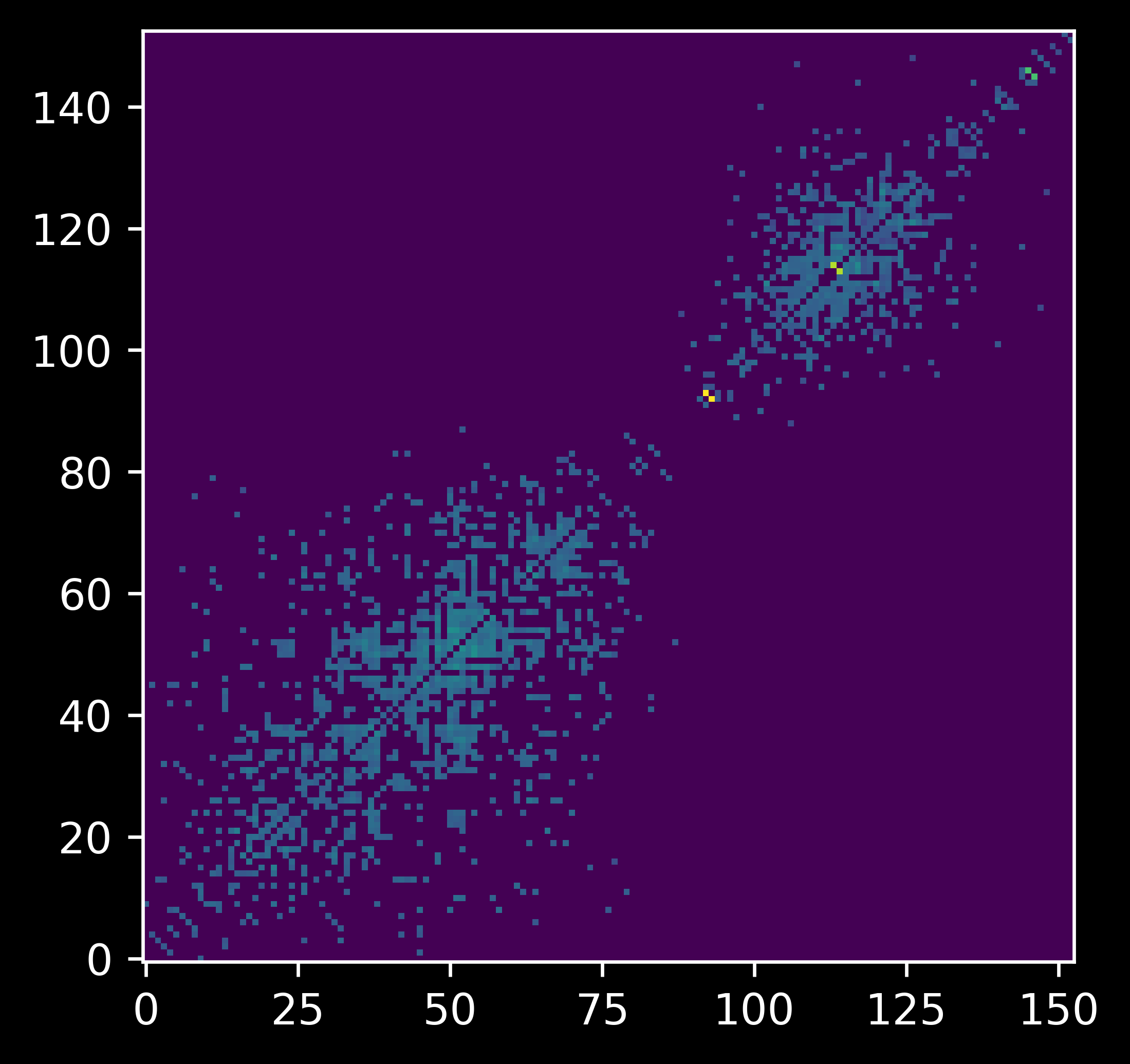
Visualisation of produced solution.
Energy: 9791.369085289818
Score: 0.7738583765846074
So, I stuck with the algorithm I had and added a few minor optimisations to allow it to run slightly faster:
- I gave the simulated annealing algorithm the output from the MST-based algorithm as an initial solution, so that it did not have to start the search from scratch.
- When calculating the new energy of a solution after a random swap, I changed the code to calculate the change in energy instead, which was faster to compute.
- I made the scoring system and annealing algorithm both operate on the inverse permutation to avoid having to invert the permutation a bunch of times, since a bunch of calculations require the inverse calculated.
- Expressing the entire scoring process as a matrix multiplication and precomputing the distance and weight matrices meant that I could speed up score calculations by computing them entirely within NumPy.
Most of this I did with the help of a fellow student, Kuba. Thanks!
If you’re interested, I have also shared a Python notebook with my code on Google Colaboratory.
How did it do so well?⌗
I think it has to do with how you can get from any permutation to any other permutation in a relatively small number (at most $N-1$) of swaps. This means that the algorithm can easily get a “feel” for the entire landscape of solutions, from which it can select a promising direction to explore.
Is there any research already done on the problem?⌗
When Kuba and I were formalising the scoring process as a matrix multiplication, we realised that this problem is actually equivalent to the quadratic assignment problem, which we discovered to be NP-hard.
Not to worry, once you have a reduction to a known problem, there is normally still a well-studied algorithm for the problem that produces a pretty good solution. QAP is not an exception! It turns out, SciPy has a solver for it! Let’s plug it in and see what score it gets:
0.7626726033749955
…oh. Our solution performed better than the SciPy solver. To be fair, 76% is still very impressive, but my simulated annealing algorithm achieved 77% by leveraging extra computation time.
Act III - Epilogue⌗
There were still so many loose ends! For one, my lecturer had hinted at max-flow for being one of the potential paths to explore for tackling this problem. What? This isn’t max-flow at all!
I emailed my lecturer about my findings. This is what he had to say:
The best way to score well on this challenge is definitely to use randomized optimization methods such as simulated annealing. There is no “classic” algorithm (that I’m aware of) that works as well.
My comment about max-flow is “Do you have the out-of-the-box thinking needed to turn a problem of one sort into a problem of another sort?” (Hardly anyone in CS ever thinks about Kruskal’s algorithm as a tool for clustering – but if you just look at Kruskal slightly differently, it’s obviously usable for that data analysis task.) For this challenge this out-of-the-box thinking hasn’t led me to a better algorithm; as I said, randomized methods work best here. But the journey is more interesting than the destination! Maybe wait until Friday’s lecture, and after that see if any further thoughts about max-flow come to you. In general, if you’re the fastest person to spot “hey, we could try to solve problem X by reformulating it as Y”, then you’ll have a serious advantage in research and in life!
Oh, right. The purpose of this challenge was to draw connections. What connections did we draw for this problem?
- We turned the scoring formula of the problem into a series of matrix multiplications.
- The series of matrix multiplications allowed us to show that it was equivalent to the quadratic assignment problem, and hence show that it was NP-hard.
At the end of the day, even though the approach I took had nothing to do with max-flow, I still ended up drawing a lot of connections between different concepts in computer science. More importantly, I learned that many problems can leverage solutions to known problems to craft decent solvers without much effort.